Is the Fed Model fit only for statistics-challenged practitioners, or does it offer some trading intelligence? In the January 2007 version of his paper entitled “A Behavioral Defense of the Fed Model”, Michael Clemens combines the concepts of mean reversion of key financial variables and confidence intervals to present a behavioral defense of the Fed model. He examines the version of the model based on the spread between the S&P 500 forward earnings yield (E/P) and the yield on the 10-year Treasury note. His defense includes identification of ten potential chinks in the armor of model detractors. Using monthly data for the period January 1979 through August 2006 (322 monthly observations over 26 years) , he finds that:
- The Fed model detects time variation in the equity risk premium and behavioral biases in long-term earnings growth expectations.
- Incorporating confidence intervals (margins of safety) into a Fed model-based trading decision process reduces the risk of bad decisions triggered by noise or sentiment. The Fed model works best when the yield spread is outside some reasonable confidence interval (for example ±1.5 standard deviations).
- The Fed model predicts the relative return of stocks versus bonds better than it predicts absolute stock returns.
- The optimal prediction horizon for the Fed model is in the range 12-36 months.
- The Fed model is slightly more reliable for predicting stock market downturns than upturns.
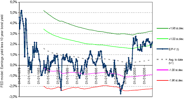
The following figure, taken from the paper, shows the behavior of the Fed model yield spread and associated simple statistics since the beginning of 1979. The author finds that the distribution of the yield spread over time is close enough to normal to warrant the use of standard normal distribution statistics. He calculates the average and standard deviations from the beginning of the overall sample to one month before each yield spread measurement. Each point on the yield curve graph is therefore out-of-sample with respect to these statistics. The figure indicates that the mean yield spread is fairly stable over time. It also shows that there have been only two opportunities to act at a 95% confidence level (+/- 1.96 standard deviations) in recent decades.

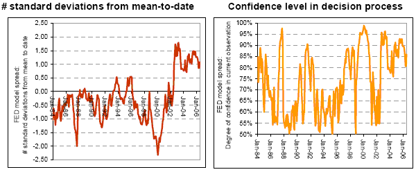
The next two figures, also from the paper, encapsulate a Fed model-based decision process using confidence intervals. Using data from the preceding figure, the left side depicts the yield spread in number of standard deviations above or below a running to-date mean. The right side translates standard deviations into confidence intervals (assuming the underlying distribution is normal). A confidence level of 50% (90%) indicates a 50% (10%) risk of being wrong in positioning for mean reversion.

In summary, the Fed model and the long-term P/E mean reversion model are complementary perspectives on return prediction, with the former reasonably useful for forecasting up to three years into the future and the latter applicable over longer horizons.
As often found in financial forecasting analyses, and as acknowledged by the author, operating at a high confidence level means compressing sample size to an unusably low count and almost never getting trading signals (no risk = paralysis). For example, the 24 observations (months) outside ±1.5 standard deviation bands lie in just five clusters (consecutive-month signals). The use of monthly input data with multi-year prediction horizons tends to overstate true sample size. Even without any sample size illusion, a trader could in general apply available capital only once per cluster, representing five (not 24) trading opportunities with fairly high confidence of mean reversion over 26 years.