Does the set of variables that have the strongest correlations with subsequent U.S. stock market returns over the prior decade usefully predict market returns out-of-sample? In the July 2015 draft of their paper entitled “A Practitioner’s Defense of Return Predictability”, Blair Hull and Xiao Qiao apply this correlation screening approach to a set of 20 published stock market forecasting variables encompassing technical indicators, macroeconomic variables, return-based predictors, price ratios and commodity prices. Their horizon for historical daily correlation measurements and out-of-sample forecasts is 130 trading days (about six months). Every 20 days just before the market close, they employ regressions using the most recent ten years of data to: (1) determine the form of each forecasting variable (raw value, exponentially-weighted moving average or log value minus exponentially-weight moving average) that maximizes its daily correlation with 130-day returns; and, (2) estimate variable coefficients to predict the return for the next 130 days. For the next 20 days, they then use the estimated coefficients to generate expected returns and take a (market on close) position in SPDR S&P 500 (SPY) eight times the expected return in excess of the risk-free rate (capped at 150% long and 50% short). They consider three expected return models:
- Kitchen sink – employing regression coefficients for all 20 forecasting variables (but with four of the variables compressed into a composite).
- Correlation Screening – employing regression coefficients only for forecasting variables having absolute correlations with subsequent 130-day market returns at least 0.10 over the past ten years.
- Real-time Correlation Screening – same as Correlation Screening, but excluding any forecasting variables not yet discovered (published).
They assume: trading frictions of two cents per share of SPY bought or sold; daily return on cash of the three-month U.S. Treasury bill yield minus 0.3%; and, interest on borrowed shares of the Federal Funds Rate plus 0.3%. To limit trading frictions, they adjust positions only when changes in expected market return reach a threshold of 10%. They ignore tax implications of trading. Using daily total returns for SPY, the 3-month Treasury bill yield and vintage (as-released) values of the 20 forecast variables during 6/8/1990 through 5/4/2015, they find that:
- Over a test period starting in June 2001 and ending in early May 2015:
- The Kitchen Sink market timing model generates an annualized return similar to that of buy-and-hold (5.9% versus 5.8%), but with a much higher Sharpe ratio (0.41 versus 0.21) and a smaller maximum drawdown (-26% versus -55%).
- The Correlation Screening model easily outperforms buy-and-hold based on annualized return (12.1%), Sharpe ratio (0.85) and maximum drawdown (-21%). Average equity exposure is around 60%. The strategy underperforms the market in seven of 15 years.
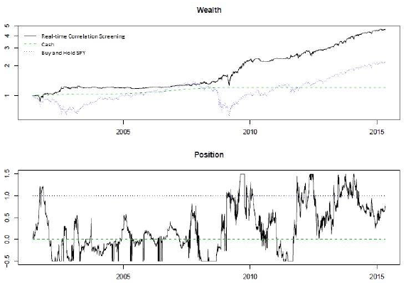
- Real-time Correlation Screening model performance is similar to that of the Correlation Screening model (see the charts below): annualized return 11.7%, Sharpe ratio 0.88 and maximum drawdown -22%. It underperforms the market in six of 15 years.
- While the correlation-screened market timing strategies outperform the market, they are difficult to implement and would be substantially eroded by taxes unless sheltered in retirement accounts or foundations.
The following charts, taken from the paper, compare: (1) cumulative performances of the Real-time Correlation Screening market timing strategy and buying and holding SPY (upper chart); and, (2) the dynamic positions in SPY of the Real-time Correlation Screening market timing strategy capped at 150% long and 50% short (lower chart). The timing strategy easily outperforms buy-and-hold over the entire test period, with outperformance concentrating during the two bear markets. During bull markets, the timing strategy approximately matches or underperforms buy-and-hold.
In summary, evidence indicates that elaborate strategies combining many U.S. stock market forecasting variables may support economically significant market timing by avoiding most of bear markets.
Cautions regarding findings include:
- As noted, the forecasting methodology and data requirements are complex. Data acquisition/processing and position adjustments on the tight schedule assumed may be problematic. Most investors would have to delegate this work and pay management fees.
- The complex methodology has many parameters (20-day iteration cycle, 10-year lookback interval, 130-day forecast horizon, position size eight times expected return, 10% adjustment threshold for changes in expected return, levels of trading/shorting frictions and return on cash, leverage limits). For regression parameters, the authors report that other combinations generate similar results. However, there may be residual data snooping bias in outcomes.
- As noted in the paper, the sample period includes deep bear markets in 2002 and 2008 that are important to timing strategy outperformance. It is unusual for two such deep downturns to occur only six years apart.
- The assumed levels of trading frictions and shorting costs may be low for many investors.
- As noted, results do not account for taxes.