Do quantitatively-driven mutual fund managers such as John P. Hussman, Ph.D, president of Hussman Investment Trust, successfully time the stock market? He describes his market timing approach as follows: “The key elements in evaluating securities and market conditions are ‘valuations’ and ‘market action.’ Each unique combination of these conditions results in a distinct Market Climate, with its own profile of expected return and risk.” His investment approach, as applied to funds such as Hussman Strategic Growth (HSGFX), is to “align our investment position with the prevailing Market Climate and shift that position when sufficient evidence of a Climate shift emerges.” Does this fund demonstrate good market timing? Using weekly dividend-adjusted returns for HSGFX during 11/21/00 (the earliest available) through 7/26/13 (660 weekly returns), along with contemporaneous weekly returns for the S&P 500 Index and the Russell 2000 Index as benchmarks, we find that:
Each of the Hussman funds “varies its exposure to market fluctuations – from neutral to aggressive – based on the unique return/risk characteristics of each Market Climate”. Performance of such a fund with respect to some index, such as the S&P 500 Index, therefore derives from some combination of:
- Stock selection (including dividends).
- General policy to hedge exposure of the selected portfolio to market fluctuations.
- Hedging adjustments based on expected returns for variations in market climate (market timing).
- Trading frictions and fund fees.
If the hedging adjustments are effective, the fund portfolio should be on average more (less) sensitive to fluctuations of the broad stock market when the market advances (declines).
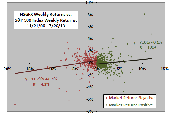
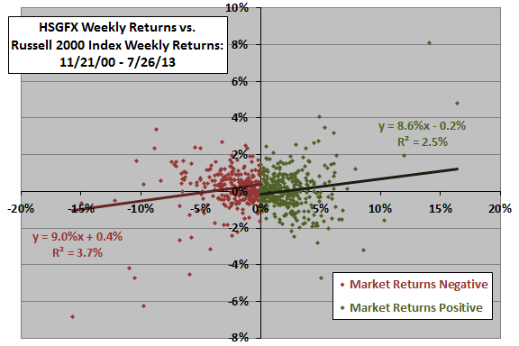
As tests of the effectiveness of HSGFX hedging adjustments, the following two scatter plots relate the weekly returns of HSGFX to those of the S&P 500 Index (upper chart) and the Russell 2000 Index (lower chart) separately when the weekly index return is negative (red) and positive (green) over the entire sample period. Each chart shows both the equations for the best-fit lines and the R-squared statistics for advancing and declining markets.
Relative to the S&P 500 Index, HSGFX is a little more sensitive to market fluctuations when the market is falling (slope or beta of 11.7% and R-squared of 4.2%) than when it is rising (beta of 7.3% and R-squared of 1.3%). In other words, efforts to time the market by adjusting the level of hedging appear to harm the fund’s long-run performance.
Relative to the Russell 2000 Index, HSGFX is about equally sensitive to market fluctuations when the market is falling (beta of 9.0% and R-squared of 3.7%) and when it is rising (beta of 8.6% and R-squared of 2.5%). In other words, efforts to time the market by adjusting the level of hedging appear to have no effect on the fund’s long-run performance.
For both charts, the y-intercept or weekly alpha is positive (a little negative) when the broad market is falling (rising), indicating that benefit of stock selection derives mostly from intervals of broad market weakness (portfolio stock holdings are defensive). Alpha is positive in the first half of the sample period (0.22% weekly) and negative in the second half (-0.06% weekly).
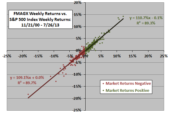
For comparison, we replicate this analysis for a conventional, unhedged mutual fund.
The next scatter plot relates the dividend-adjusted weekly returns of Fidelity Magellan (FMAGX) to those of the S&P 500 Index separately when the weekly index return is negative (red) and positive (green) over the entire sample period. Results show that the exposure of FMAGX to market fluctuations is about the same whether the broad market is rising or falling, and that it is far more sensitive to these fluctuations than is the HSGFX portfolio. The R-squared statistics indicate that broad market fluctuations explain nearly 90% of the variation in FMAGX returns. Note that the y-intercept or alpha is little different from zero when the market is falling or rising.
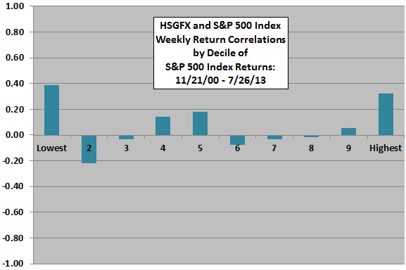
For another perspective on the HSGFX timing effectiveness, we look at correlations between HSGFX and S&P 500 Index weekly returns by range of the latter.
The next chart summarizes the correlations between HSGFX and S&P 500 Index weekly returns by ranked tenth (decile) of S&P 500 Index returns over the entire sample period. A steadily increasing progression of correlations across deciles would indicate systematically good timing, but no such progression is evident. In fact, HSGFX appears just as exposed to extremely negative market returns as it is to extremely positive market returns.
How does the correlation between HSGFX and S&P 500 Index returns vary over time?
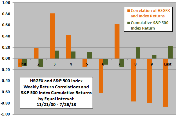
The next chart shows the correlations between between HSGFX and S&P 500 Index weekly returns (orange columns) and cumulative S&P 500 Index returns (green columns) over ten equal, consecutive subperiods (each roughly 16 months long). When these two series have the same sign (opposite signs), timing via hedging adjustments is favorable (unfavorable). Results indicate that timing is favorable in only four of ten subperiods. Timing is unfavorable in each of the last four subperiods.
For another perspective on the role of hedging (not timing), we look at average weekly returns.
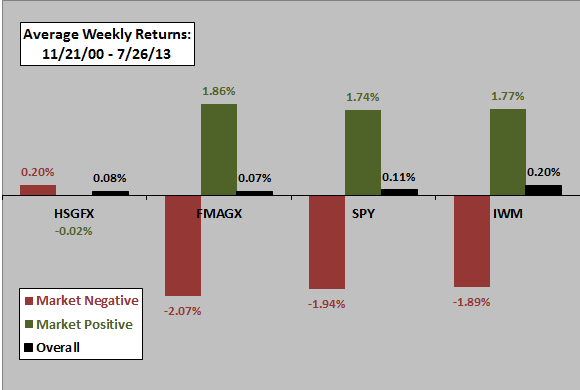
The final chart compares average weekly total returns for HSGFX, FMAGX, S&P Depository Receipts (SPY) and the iShares Russell 2000 Index (IWM) when the weekly S&P 500 Index return is negative (red), positive (green) and overall (black) for the entire sample period. The chart shows that, while FMAGX closely mimics SPY behavior, HSGFX on average avoids market weakness but also misses market strength. Cumulative returns over the entire sample period (ignoring tax implications) are 62%, 22%, 59% and 161%, respectively, for HSGFX, FMAGX, SPY and IWM.
In general, when the mix of up and down market weeks tilts substantially toward down (up) intervals, HSGFX tends to do relatively well (poorly). During the sample period, there are 360 (54.5%) up weeks and 300 down weeks (45.5%) for the S&P 500 Index. Since the beginning of 1950, the S&P 500 Index has 56.6% up weeks and 43.4% down weeks.
The hedging approach suppresses portfolio volatility considerably. The standard deviations of weekly returns are 1.1%, 2.9%, 2.6% and 3.3%, respectively, for HSGFX, FMAGX, SPY and IWM over the entire sample period, yielding weekly return-risk ratios of 0.07, 0.03, 0.04 and 0.06.
In summary, evidence from simple tests does not support belief that John Hussman successfully times the stock market via fund hedging adjustments based on his assessments of market valuation and market action.
Cautions regarding findings include:
- The sample period is not long in terms of number of bull and bear markets.
- Returns for the S&P 500 Index and the Russell 2000 Index do not account for dividends.
Findings are generally consistent with those described in “Outperformance of Hedge Funds: Timing or Asset Selection?”, “Hedge Fund Success: Timing or Stock Picking?” and “Mutual Fund Stock Selection vs. Market Timing” that funds do not time the market effectively.