Does timing the U.S. stock market with moving averages work? In his October 2015 paper entitled “A Comprehensive Look at the Real-Life Performance of Moving Average Trading Strategies”, Valeriy Zakamulin employs a very long dataset to estimate out-of-sample performance and robustness (subsample performance) of four distinct technical trading rules. Specifically, he seeks answers to the following questions:
- How well does market timing really work?
- Does overweighting or underweighting recent prices improve market timing?
- Do timing rules have optimal lookback intervals?
- Can timing rules accurately exploit bull and bear market states?
The four trading rules are:
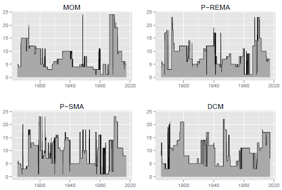
- Momentum (MOM) – final price minus initial price across the measurement interval.
- Price minus Simple Moving-Average (P-SMA) – final price minus linearly decreasing weighted average of past prices backward over the measurement interval.
- Price minus Reverse Exponential Moving Average (P-REMA) – final price minus exponentially decreasing weighted average of past prices with decay factor 0.8, for an effect between MOM and P-SMA.
- Double-Crossover Method (DCM) – long-interval EMA minus short-interval EMA with decay factors 0.8 and the short interval fixed at two months.
For all four rules, a positive (negative or zero) signal means hold stocks (the risk-free asset) the following month. For optimization of moving average lookback intervals, he considers both rolling 10-year windows and inception-to-date (expanding window) data and tests intervals up to 24 months. His total sample spans 1860 through 2014, with the first 10 years reserved for lookback interval optimization. He also considers two equal subsamples (1860-1942 and 1932-2014), with the first 10 years of each reserved for initial optimization. He assumes one-way switching friction 0.25%. He uses several risk-adjusted performance measures, emphasizing Sharpe ratio. Using monthly capital gains and total returns of the S&P Composite stock price index and the contemporaneous U.S. Treasury bill yield as the risk-free rate during January 1860 through December 2014, he finds that:
- Average monthly total index return over the entire out-of-sample (commencing 1870) period is 0.85%, with standard deviation 4.99%. Average return is lower (0.70% versus 1.01%) and more volatile (5.70% versus 4.16%) for the first half compared to the second half.
- Over the entire sample period, as delineated by highest local maximums and lowest local minimums, there are 41 (40) bull (bear) markets, with average duration 29.3 (15.5) months and average return +65% (-24%).
- For 10-year rolling windows, average optimal (maximum Sharpe ratio) lookback intervals range from 8.1 months for MOM to 9.7 months for P-SMA. However:
- Optimal intervals vary widely and frequently (see charts below).
- Average optimal lookback intervals are mostly shorter for the second half of the sample than for the first half.
- Based on Sharpe ratios, every timing strategy beats the market over the entire sample period and the two subperiods because reductions in mean returns are less than reductions in volatilities. However:
- Over the entire period, only MOM and P-REMA based on rolling window optimization exhibit statistically superior performance.
- Over the first subperiod, only MOM based on rolling window optimization exhibits statistically superior performance.
- Over the second subperiod, while timing strategies have Sharpe ratios 7% to 14% higher than the market, none exhibit statistically superior performance.
- In general, evidence does not support belief that overweighting recent prices improves moving average rule performance.
- In general, differences in performance between rolling window and expanding window optimizations is small (with the former generating more trades).
- Over the entire sample period, timing rules are only slighting more accurate (by 1% to 3%) than buy-and-hold in predicting market state (bull or bear). Moreover:
- Timing rules have negative average returns during bear markets.
- Timing rules tend to capture the biggest down months but exclude the biggest up months in the stock market.
- Outperformance of market timing rules comes mostly from bear markets during the 1870s, 1900s, 1930s, 1970s and 2000s. Moreover:
- Timing rules sometimes underperform for decades. For example, P-SMA underperforms from the early 1930s to the late 1960s and from the late 1970s to the early 2000s.
- Only MOM beats the market in more than 50% of 5-year intervals.
- Performance of market timing rules deteriorates over time.
- Results are similar for different risk adjustment metrics and for all rolling window lengths exceeding five years.
The following charts, taken from the paper, show optimal lookback intervals in months for the four specified technical trading rules over rolling 10-year historical windows (the first measurement covers January 1860 through December 1869). Wide and frequent swings in optimal intervals undermine belief that optimality is reliable.
In summary, evidence provides some support for belief that U.S. stock market timing based on moving averages improves risk-adjusted investment performance, but support comes mainly from the 1860-1942 subsample.
Cautions regarding findings include:
- There may be data quality issues due to use of approximations/modeling in constructing the long price series.
- Testing many alternative rules on the same data introduces data snooping bias, such that the best-performing rule overstates expected Sharpe ratio. Since the number of rules tested is known and fairly small, the study could explicitly correct for this bias.
- Data may not have been available in a timely manner as assumed over much of the sample period, making a part of backtests unrealistic.
- As noted in the paper, findings may differ for price measurement frequencies other than monthly.
- As noted in the paper, findings may differ for other asset price series due to inherently different behaviors (see, for example, “Optimal Intrinsic Momentum and SMA Intervals Across Asset Classes” and“SMA Signal Effectiveness Across Stock ETFs”).
- Use of an index ignores the costs of maintaining a tradable tracking fund. Incorporating such costs would lower all reported Sharpe ratios. Also, the existence of such a fund during the entire sample period may have altered investor behavior.
- The assumed 0.25% switching friction is arguably much too low for large parts of the sample period (see “Trading Frictions Over the Long Run”) and too high for recent data.
See the closely related “Best Moving Average Weighting Scheme for Market Timing?”.