Does trading based on simple moving average crossings reliably improve the performance of a portfolio diversified across asset classes? In the February 2013 update of his paper entitled “A Quantitative Approach to Tactical Asset Allocation”, Mebane Faber examines the effects of applying a 10-month simple moving average (SMA10) timing rule separately to each of the following five total return indexes a part of an equally weighted, monthly rebalanced portfolio: (1) S&P 500 Index; (2) 10-Year Treasury note constant duration index; (3) MSCI EAFE international developed markets index; (4) Goldman Sachs Commodity Index (GSCI); and, (5) National Association of Real Estate Investment Trusts index. Specifically, at the end of each month, he enters from cash (exits to cash) any index crossing above (below) its SMA10. Entry and exit dates are the same a signal dates (requiring some anticipation of signals before the close). The return on cash is the 90-day Treasury bill (T-bill) yield. Calculations ignore trading frictions and tax implications. Using monthly total return series for selected indexes mostly during 1972 through 2012, he finds that:
- Applied to the total return S&P 500 Index alone:
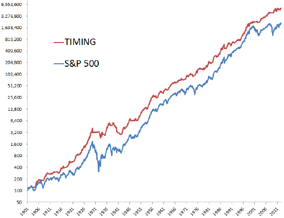
- During 1901 through 2012, the SMA10 timing rule (buy-and-hold) generates a gross annualized return of 10.2% (9.3%), with annual standard deviation 12.0% (17.9%). The corresponding gross annualized Sharpe ratio is 0.55 (0.32), and the maximum annual drawdown is -50.3% (-83.5%). (See the first chart below.)
- During 1990-2012, the SMA10 timing rule exhibits substantial gross outperformance compared to buy-and-hold.
- Applied separately to each of the five indexes specified above as part of an equally weighted, monthly rebalanced portfolio:
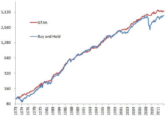
- During 1973 through 2012, the SMA10 timing rule (buy-and-hold) generates a gross annualized return of 10.5% (9.9%), with annual standard deviation 7.0% (10.3%). The corresponding gross annualized Sharpe ratio is 0.73 (0.44), and the maximum annual drawdown is -9.5% (-46.0%). (See the second chart below.)
- The model is at least 60% invested about 80% of the time, with overall average investment level 70% (30% cash).
- Based on gross Sharpe ratio, timing robustly beats buy-and-hold for 3-month, 6-month, 9-month and 12-month SMAs.
- During 2006 through 2012 (since publication of the model), although winning only three of seven years, the SMA10 timing model (buy-and-hold) generates a gross annualized return of 10.5% (9.9%), with annual standard deviation 6.0% (3.9%). The corresponding gross annualized Sharpe ratio is 0.61 (0.16), and the maximum annual drawdown is -9.5% (-46.0%).
- Due to the low turnover of the model (three to four round-trip trades per year for the five-asset portfolio), trading friction would be low. The impact of taxes (unless sheltered) would be material, but the model generates mostly long-term capital gains.
- Expanding the set of indexes to 13, with four U.S. equity styles (based on size and momentum), developed and emerging international equities, four categories of bonds, GSCI, gold and real estate:
- During 1973 through 2012, the SMA10 timing model applied to the 13 assets (original five) generates a gross annualized return of 12.0% (10.5%), with annual standard deviation 7.1% (7.0%). The corresponding gross annualized Sharpe ratio is 0.94 (0.73), and the maximum annual drawdown is -10.7% (-9.5%).
- Putting cash into a 10-year U.S. Treasury note index rather than 90-day T-bills boosts gross annualized return to 13.4% and gross annualized Sharpe ratio to 0.98.
- Portfolio weighting refinements can boost the gross annualized Sharpe ratio over one.
The following chart, taken from the paper, compares on a log scale the gross cumulative performances of buying and holding the total return S&P 500 Index (S&P 500) and applying the SMA10 timing rule (TIMING) to the index during 1901 through 2012. The timing rule outperforms largely by avoiding most of the drawdowns of major bear markets. There appears to be, however, a long subperiods (1940-2000) when the timing rule does not widen the gap with buy-and-hold.
The next chart, also from the paper, compares on a log scale the the gross cumulative performances of holding an equally weighted, monthly rebalanced portfolio of the five asset class proxies specified above (Buy and Hold) and applying the SMA10 timing rule separately to each of the indexes within the portfolio (TIMING) during 1973 through 2012. The timing rule outperforms largely by avoiding most of the severe drawdown of 2008. Such unusual conditions may be critical to model outperformance.
In summary, evidence indicates that an SMA-based trend-following rule applied separately to each of several asset class proxies within a diversified portfolio substantially enhances gross risk-adjusted performance by avoiding episodes of downside volatility.
See Cambria Global Tactical ETF (GTAA) for a recent, related (but more complex) implementation of the tested model via an exchange-traded fund (ETF).
Cautions regarding findings include:
- Reported returns are gross of trading frictions incurred via the SMA10 rule and monthly rebalancing of multi-asset portfolios. Including reasonable estimates of trading frictions, which vary considerably over the sample period (see “Trading Frictions Over the Long Run”) and likely by asset class, would reduce these returns. For a current implementation, as asserted in the paper, trading frictions generated by the SMA10 rule would be small. Monthly rebalancing of the multi-asset portfolio may still generate material frictions depending on broker fee and account size.
- The use of indexes rather than tradable assets omits the management, administrative and trading costs associated with creating a tradable asset from a collection of securities. These costs vary over time and across asset classes. In recent times, these costs are relatively small.
- Data snooping bias via selection of a 10-month SMA may be material for U.S. stocks (see “Is There a Best SMA Calculation Interval for Long-term Crossing Signals?” and “10-Month SMA Reputation a Data Mining Artifact?”)
- As noted, substantial outperformance of the multi-class implementation relative to passive equal weighting may depend on rare conditions such as those encountered in 2008.
Intrinsic (or absolute) momentum is an alternative to the SMA10 rule as a signal for entering/exiting each asset. See, for example, “Intrinsic Momentum Across Asset Classes”, “Intrinsic Momentum Framed as Stop-loss/Re-entry Rules”, “Intrinsic Momentum Versus SMAs for Size Portfolios” and “Intrinsic Momentum or SMA for Avoiding Crashes?”.