Reader Richard Beddard, editor of Interactive Investor, flagged a series of three studies by Keith Anderson and Chris Brooks on approaches to enhancing the value premium via empirical analysis of the price-earnings ratio (P/E) calculated with lagged earnings. One study seeks to optimize value indication based on the extent and weighting of historical earnings used in the P/E calculation. The second study seeks to concentrate the value premium by decomposing P/E into components related to market, firm size, industry and company-specific factors. The third study combines the findings of the first two and examines the returns for the extreme tails of the enhanced P/E distribution. All three studies use earnings and stock return data for a broad range of UK companies (excluding the smallest) for the period 1975-2004. Summaries of the three studies follow.
In the May 2005 paper entitled “The Long-Term Price-Earnings Ratio”, the authors seek to maximize the value premium indicated by P/E based on the amount and weighting of historical earnings applied in calculating it. They find that:
- P/E based on one-year trailing earnings results in an average annual value premium of about 6% between the 10% of stocks with the lowest P/Es (value) and 10% of stocks with the highest P/Es (glamour, or growth).
- Compared to P/E based on one year of history, P/E based on average earnings over the last:
- Two or three years reduces this value premium.
- Four or five years produces about the same value premium.
- Six to eight years increases this value premium.
- Eight years nearly doubles the value premium (to 11.7%).
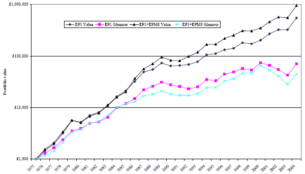
- Among simple weighting systems, calculating P/E based with straight-line reverse weighting of eight years of historical earnings (oldest weighted heaviest) indicates the highest value premium (12.2%). Calculating P/E by adding last year’s earnings to those from eight years ago (ignoring the six years in between) indicates an even higher value premium of 12.7% (see chart below).
- Results are robust across subperiods and to potential differences in transaction costs for value and glamour portfolios. Liquidity may be an obstacle for institutional investors when buying small-capitalization stocks.
The following chart, taken from the paper, shows the cumulative value on a log scale during 1975-2004 of initial £1,000 investments in the 10% of stocks with the lowest P/Es (value) and the 10% with the highest P/Es (glamour, or growth), rebalanced annually. Value based on P/Es calculated with last year’s earnings plus those from eight years ago (EP1+EPM8) outperforms value based on P/Es calculated with just last year’s earnings (EP1). And, glamour defined based on (EP1+EPM8) underperforms glamour based on EP1 alone. Over 29 years, the (EP1+EPM8) value portfolio is worth almost twice the EP1 value portfolio, while the (EP1+EPM8) glamour portfolio is worth only two-thirds the EP1 glamour portfolio. The average annual value premium is 12.7% for (EP1+EPM8) versus about 6% for EP1.

In summary, careful parsing of earnings history can enhance the use of historical P/E as an indicator of the value premium.
In the May 2005 paper entitled “Decomposing the Price-Earnings Ratio”, the authors test the value premium discrimination power of an adjusted P/E derived from: (1) the contemporaneous market P/E (reflecting shifts in aggregate investor confidence); (2) firm size (small companies tend to have lower P/Es); (3) the industry in which the company operates (there is wide variation of average P/Es across industries); and, (4) idiosyncratic effects of unique company information. They find that:
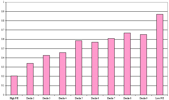
- The adjusted P/E has strong discriminating power based on both returns and Sharpe ratio (see chart below).
- The market capitalization adjustment factor has the largest effect, increasing the likelihood that shares of small firms are designated as value stocks (in effect, combining the size effect and the value premium). However, accounting for the larger bid-ask spreads of small stocks eliminates most of this effect.
- The adjusted P/E doubles the gap in annual returns between the 10% of stocks with the lowest P/Es (value) and the 10% with the highest P/Es (glamour, or growth), from 5.25% to 10.5%.
- A portfolio of value (glamour, or growth) stocks selected via adjusted P/E outperforms (underperforms) a portfolio selected via traditional P/E by 2.4% (-2.7%) annually. Over 30 years, rebalanced annually, the adjusted value portfolio ends up being worth almost double the traditional value portfolio. A hedged portfolio that is long value and short glamour based on adjusted (traditional) P/E has seven (13) down years out of 30.
- P/E adjustments are reasonably stable across subperiods.
The following chart, taken from the paper, illustrates the value-discrimination power of adjusted P/E in terms of Sharpe ratio (using the 3-month Treasury bill yield as the risk-free rate). The Sharpe ratio for the 10% of stocks with the lowest adjusted P/Es (value) is about four times that of the 10% with the highest adjusted P/Es (glamour, or growth), and Sharpe ratios generally increase as adjusted P/E decreases. Although the variability of returns is somewhat higher for low P/E stocks, the standard deviation does not rise as quickly as the returns.

In summary, adjusting P/E to account for market, industry and style factors enhances its power as a value indicator.
In the April 2005 paper entitled “Extreme Returns from Extreme Value Stocks: Enhancing the Value Premium”, the authors extend the above findings to test whether the very best (worst) returns are concentrated among a very few stocks with the very lowest (highest) P/Es. For this analysis, they use eight years of company earnings history to measure long-term earnings power. Also, they strip away the predictable influences of the overall market, firm size and industry to focus on the idiosyncratic (firm-specific) component of each company’s P/E. They find that:
- Small portfolios of very low adjusted P/E (extreme value) stocks yield returns of over 40% annually. Small portfolios of very high adjusted P/E (extreme glamour, or growth) stocks yield returns less than the risk-free rate. The associated value premium exceeds 30% per year.
- Despite having very high standard deviations, the returns for small extreme value portfolios are so large that their Sharpe ratios are the highest. The returns on small extreme glamour portfolios are less variable, but their returns are extraordinarily bad, producing extremely poor Sharpe ratios.
- The average returns for extreme value portfolios rise from 30% to over 40% as the number of stocks held declines from 15 to five. The Sharpe ratio declines for extreme value portfolios of fewer than six stocks. For a hedged portfolio that is long extreme value and short extreme glamour, six stocks for each category is optimum.
- Extreme value returns are so large that data snooping bias is unlikely to explain them fully. A wide range of enhanced P/E trading strategies offers substantially increased value premiums.
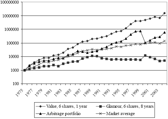
The following chart, taken from the paper, shows the cumulative value on a log scale during 1975-2004 of initial £1,000 investments in: (1) the six extreme value stocks, rebalanced annually; (2) the six extreme glamour stocks, rebalanced every eight years; (3) the arbitrage portfolio (+/- £1,000) that is long the extreme value stocks and short the extreme glamour stocks; and, (4) an equally-weighted market average for all UK stocks with eight years of positive earnings.
- The extreme value portfolio turns £1,000 in 1975 into £15 million in 2004, an annual compound rate of 39.3%. It gives returns of over 100% three times, and returns of over 50% ten times. Its only significant loss is 20% in 2002-3, from which it rebounds to more than double the following year.
- The extreme glamour portfolio generates a compound return of 5.7%, less than the average return for 3-month Treasury bills. It produces losses in 12 of 29 years.
- The arbitrage portfolio grows to £600,000 in 2004, an annual compound rate of 24.7%. It substantially underperforms the extreme value portfolio because of near catastrophe in 1999-2000, when extreme glamour stocks more than double.
The standard deviations of the three extreme portfolios are similar. The arbitrage portfolio does not hedge against overall market shocks.

In summary, an investment strategy based on extreme P/Es calculated with an extended earnings history and concentrated by stripping out market, industry and style factors offers extreme returns.
For additional summary-level information on these studies, see Dr. Anderson’s “Improving the P/E” web pages.
A reader who is a strategist at a European equity hedge fund makes the following two observations:
1. “In ‘The Long-Term Price-Earnings Ratio’, the authors conclude that low P/E companies are superior performers, but they exclude from their sample all companies that have any negative earnings between 1975 and 2003 (see page 9 of the paper). It is no surprise to see that within this biased set of ‘survivors,’ low P/E companies turn out to have been good buys.”
2. “In ‘Decomposing the Price-Earnings Ratio’, the authors present only in-sample tests. They acknowledge the issue, as follows: ‘These results can fairly be criticised as suffering from a look-ahead bias, in that the regression weights could only have been known in May 2004, but we use them to calculate annual returns for the whole dataset from 1975. We used a rolling ten-year sub-sample to check whether the results would be affected by the use of trailing windows of historical data to calculate the regression weights. We found that the returns are slightly degraded, but since the impact is not marked, to avoid repetition we do not report these results.’ It seems that these rolling ten-year checks are not pure out-of-sample tests.”
Regarding the first criticism:
On page 9 of ‘The Long-Term Price-Earnings Ratio’, the authors state that: “…the number of companies for each EPn calculation gradually reduces, as the EPS figure becomes unavailable for years further into the past, from 40,000 initially, to 16,000 that have a full eight years of positive earnings history.” In other words, for any given year, the companies in the sample have at least eight years (not 29 years) of positive earnings. On page 13, they state: “In this section, we used only the 16,000-company/year returns that have positive normalized earnings for each of the past eight years.” So, for example, a company in the sample at the beginning of 1995 has positive earnings since at least as far back as 1987. If that company has negative earnings in 1995, it would not be in the selection sample for 1996 (but could continue to penalize a portfolio formed at the beginning of 1995).
However, it does appear that survivorship bias comes into play when they use the broader sample to test the predictive power of last year’s earnings against that of earnings from prior years. In effect, they may be measuring the effect of earnings consistency or earnings cycles rather than earnings per se. In other words, it may be more important to restrict consideration to companies with at least eight years of positive earnings than it is to focus on calculating P/E based on earnings from eight years ago. However, it is then puzzling that earnings from two through five years in the past do not show a positive forecasting contribution due to earnings consistency.
The authors restrict both of the other papers to the 16,000 company/year sample. Anybody seeking to replicate their results would similarly have to restrict consideration to companies with at least eight years of past positive earnings.
Regarding the second criticism:
The limited (and unreported) out-of-sample testing relates to the idea of more formal accounting for data mining bias noted at the end of the original entry above. Out-of-sample testing is increasingly important as the risk of data mining bias grows.
The checks based on a rolling ten-year history to calculate alternative regression weights seems weak. Moreover, the use of a ten-year window in the one study, and the use of an eight-year rolling earnings history throughout the three studies, implies an independent sample much smaller than 29 (1975-2004), which is already small. As they note, they are unable to construct a larger study.
U.S. data may support a more extensive study, or at least a reasonably robust out-of-sample test.