Estimating Snooping Bias for a Multi-parameter Strategy

A subscriber flagged an apparently very attractive exchange-traded fund (ETF) momentum-volatility-correlation strategy that, as presented, generates a optimal compound annual growth rate of 45.7% with modest maximum drawdown. The strategy chooses from among the following seven ETFs:

ProShares Ultra S&P500 (SSO)
SPDR EURO STOXX 50 (FEZ)
iShares MSCI Emerging Markets (EEM)
iShares Latin America 40 (ILF)
iShares MSCI Pacific ex-Japan (EPP)
Vanguard Extended Duration Treasuries Index ETF (EDV)
iShares 1-3 Year Treasury Bond (SHY)

The steps in the strategy are, at the end of each month:

1. For the first six of the above ETFs, compute log returns over the last three months and standard deviation (volatility) of log returns over the past six months.
2. Standardize these the monthly sets of past log returns and volatilities based on their respective means and standard deviations.
3. Rank the six ETFs according to the sum of 0.75 times standardized past log return plus 0.25 times past standardized volatility.
4. Buy the top-ranked ETF for the next month.
5. However, if at the end of any month, the correlation of SSO and EDV monthly log returns over the past four months is greater than 0.75, instead buy SHY for the next month.

The developer describes this strategy as an adaptation of someone else’s strategy and notes that he has tested a number of systems. How material might the implied secondary and primary data snooping bias be in the performance of this system? To investigate, we examine the fragility of performance statistics to variation of each strategy parameter separately. As presented, the author substitutes other ETFs for the two with the shortest histories to extend the test period backward in time. We use only price histories as available for the specified ETFs, limited by EDV with inception January 2008. Using monthly adjusted closing prices for the above seven ETFs and for SPDR S&P 500 (SPY) during January 2008 through February 2014 (74 months), we find that:

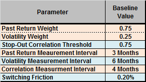
The strategy has five parameters subject to optimization: (1) past return/volatility weights; (2) stop-out correlation threshold; (3) past return measurement interval; (4) past volatility measurement interval; and, (5) past correlation measurement interval. We add switching friction to this set as a sixth parameter. The following table summarizes baseline settings for these six parameters (past return and volatility weights represent one parameter since one determines the other), all of which are optimal except for switching friction.

To test parameter measurement intervals as long as 12 months, we pick the first ETF winner in January 2009. We assume that it is possible to anticipate each monthly signal slightly such that signal and execution occur at the same close.

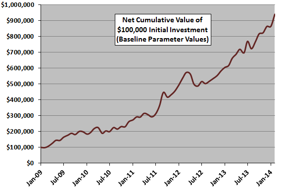
The following chart tracks cumulative value of a $100,000 investment in the strategy at the end of January 2009 with baseline parameter settings (61 monthly returns). The strategy generates 20 ETF switches over the available sample period. Terminal value is $939,634, with compound monthly growth rate (CMGR) 3.74%. Maximum peak-to-trough drawdown is -16.1%.

How sensitive are CMGR and maximum drawdown to variation in parameter settings?

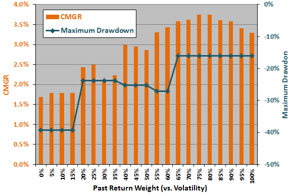
The next chart summarizes how strategy CMGR and maximum drawdown vary for past return (volatility) weights ranging from 0% (100%) to 100% (0%). In general, strategy performance is much better for high weights on past returns than for low weights.

We guesstimate a rule of thumb that the snooping bias for the optimal parameter setting is the difference between the optimal CMGR and the average CMGR for the half of the range of settings closest to the optimal setting. Here, the optimal setting is 75% or 80%, and the half of the range of settings closest to optimal is 55% to 100%. The estimated snooping bias in CMGR from past return/volatility weight optimization is therefore 0.21%.

An aggressive (conservative) investor might select a smaller (larger) range of parameter settings for guesstimating bias, thereby estimating less (more) bias. An investor who believes there is some fundamental reason why a parameter has an optimal setting may choose to ignore the effects of varying the setting.

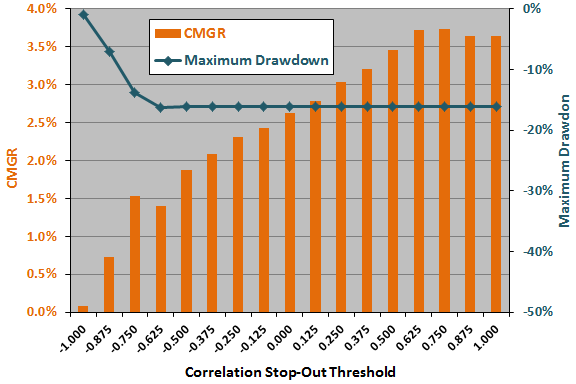
The next chart summarizes how strategy CMGR and maximum drawdown vary for correlation stop-out settings ranging from -1.000 to 1.000. In general, CMGR is much higher for high than low thresholds, though low thresholds (when SHY dominates holdings) suppress maximum drawdown.

Here, the optimal setting is 0.75, and the half of the range of settings closest to optimal is 0.125 to 1.00. Applying the above rule of thumb, the estimated snooping bias in CMGR from threshold optimization is 0.33%.

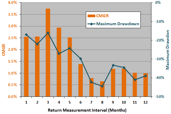
The next chart summarizes how strategy CMGR and maximum drawdown vary for past return measurement intervals ranging from one to 12 months. In general, strategy performance is much better for short than long measurement intervals. The narrowness of the optimality peak strongly suggests luck.

Here, the optimal setting is three months, and the half of the range of settings closest to optimal is one to six months. Applying the above rule of thumb, the estimated snooping bias in CMGR from return measurement interval optimization is 1.13%.

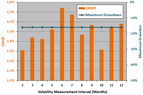
The next chart summarizes how strategy CMGR and maximum drawdown vary for past volatility measurement intervals of two to 12 months. CMGR is a little sensitive to the setting for this parameter, but maximum drawdown is insensitive. The narrowness of the optimality peak suggests luck.

Here, the optimal setting is six months, and the half of the range of settings closest to optimal is four to eight months. Applying the above rule of thumb, the estimated snooping bias in CMGR from volatility measurement interval optimization is 0.17%.

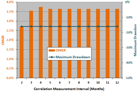
The next chart summarizes how strategy CMGR and maximum drawdown vary for past SSO-EDV return correlation measurement intervals ranging from two to 12 months. Strategy performance is insensitive to the setting for this parameter, except for the noisiest very short measurement intervals.

Here, the optimal setting is four months, and the half of the range of settings closest to optimal is two to six months. Applying the above rule of thumb, the estimated snooping bias in CMGR from correlation measurement interval optimization is therefore 0.28%.

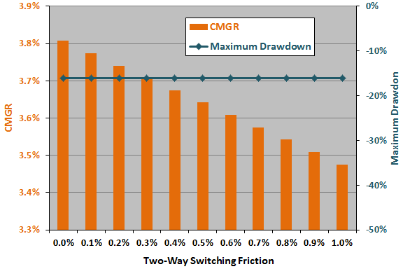
The final chart summarizes how strategy CMGR and maximum drawdown vary for two-way switching friction ranging from 0.0% to 1.0%. Obviously, CMGR degrades as friction increases, but maximum drawdown is unaffected.

The baseline friction of 0.2% is reasonable rather than optimal, and we apply no snooping bias penalty for the baseline friction setting.

Assuming the above snooping bias contributions are simply additive, the total data snooping bias penalty for CMGR is 2.13%. Subtracting this bias from the optimal 3.74% leaves 1.61%. For comparison, the CMGR for buying and holding SPY (SSO) over the bullish test period is 1.70% (2.64%). It is possible that biases from different parameters interact such that contributions are not simply additive.

In summary, investors may want to consider an approach such as the above to estimate whether the performance of a backtested strategy is strong enough to overcome potential data snooping bias.

In general, the more parameters a strategy uses, the more potential sources of data snooping bias it has. Moreover, noisy (low-confidence) parameters, such as those calculated from short historical intervals (as for the three-month past return above), tend to amplify snooping bias.

Cautions regarding findings include:

• The available sample is very short for testing the longer measurement intervals. A longer sample encompassing different market conditions would enable subperiod tests of optimal parameter settings. Consistency of optimal settings across subperiods would mitigate concern about data snooping bias.
• As noted, discovery and independent testing of fundamental reasons why an optimal setting is optimal would mitigate concern about data snooping bias.
• As noted, the biases involved in optimizing multiple parameters could interact, such that the combination would not be a simple sum.
• The above approach is illustrative. Some other way of estimating potential snooping bias may produce different results. For examples, see “Avoiding or Mitigating Snooping Bias”.
• The above analysis does not consider potential look-ahead bias in selecting a universe of ETFs after knowing their individual past performances. This kind of bias is perhaps best addressed by choosing a performance benchmark representative of the universe.