Momentum Investing

Which equity factors from among those included in the most widely accepted factor models are really important? In their October 2019 paper entitled “Winners from Winners: A Tale of Risk Factors”, Siddhartha Chib, Lingxiao Zhao, Dashan Huang and Guofu Zhou examine what set of equity factors from among the 12 used in four models with wide acceptance best explain behaviors of U.S. stocks. Their starting point is therefore the following market, fundamental and behavioral factors:

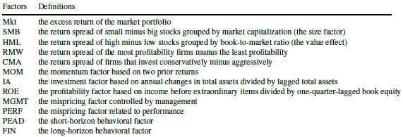
They compare 4,095 subsets (models) of these 12 factors models based on: Bayesian posterior probability; out-of-sample return forecasting performance; gross Sharpe ratios of the optimal mean variance factor portfolio; and, ability to explain various stock return anomalies. Using monthly data for the selected factors during January 1974 through December 2018, with the first 10 (last 12) months reserved for Bayesian prior training (out-of-sample testing), they find that: Keep Reading

Do U.S. equity exchange-traded funds (ETF) exhibit long-term momentum? In their October 2019 paper entitled “ETF Momentum”, Frank Li, Melvyn Teo and Chloe Yang investigate future performance of U.S. equity ETFs sorted on multi-year past returns. Each month starting August 2004, they:

1. Sort selected ETFs into tenths (deciles) based on returns over the past two, three or four years, with focus on three years.
2. Reform an equal-weighted (EW) or value-weighted (VW) portfolio that is long (short) the decile with the highest (lowest) past returns, with focus on value-weighted.

They then evaluate performances of deciles and long-short portfolios based on raw return, 4-factor (adjusting for market, size, book-to-market and momentum) alpha and 5-factor (replacing momentum with profitability and investment) alpha. Using monthly returns, market capitalizations and net asset values for all U.S. equity ETFs with capitalizations greater than $20 million and share price greater than one dollar during August 2000 through June 2018, they find that: Keep Reading

Does including a measure of asset valuation as a qualifier improve the performance of intrinsic (absolute or time series) momentum? In their October 2019 paper entitled “Carry and Time-Series Momentum: A Match Made in Heaven”, Marat Molyboga, Junkai Qian and Chaohua He investigate modification of an intrinsic momentum strategy as applied to futures using the sign of the basis (difference between nearest and next-nearest futures prices) for four asset classes: equity indexes (12 series), fixed income (18 series), currencies (7 series) and commodities (28 series). Their benchmark intrinsic momentum strategy is long (short) assets with positive (negative) returns over the last 12 months, with either: (1) equal allocations to assets, or (2) dynamic allocations that each month target 40% annualized volatility for each contract series. The modified strategy limits long (short) positions to assets with positive (negative) prior-month basis. They account for frictions due to portfolio rebalancing and rolling of contracts using cost estimates from a prior study. They focus on Sharpe ratio to assess strategy performance. Using monthly returns for 65 relatively liquid futures contract series during January 1975 through December 2016, they find that:

Keep Reading

The Simple Asset Class ETF Momentum Strategy (SACEMS) each month picks the one, two or three of nine asset class proxies with the highest cumulative total returns over a specified lookback interval. A subscriber proposed instead using the optimal intrinsic (time series or absolute) momentum lookback interval for each asset rather than a common lookback interval for all assets. SACEMS and the proposed approach represent different beliefs (which could both be somewhat true), as follows:

• Many investors adjust asset class allocations with some regularity, such that behaviors of classes are important and coordinated.
• Many investors switch between specific asset classes and cash with some regularity, such that each class may exhibit distinct times series behavior. 

To investigate, we consider two ways to measure intrinsic momentum for each asset class proxy:

1. Correlation between next-month return and average monthly return over the past one to 12 months. The lookback interval with the highest correlation has the strongest (linear) relationship between past and future returns and is optimal.
2. Intrinsic momentum, measured as compound annual growth rate (CAGR) for a strategy that is in the asset (cash) when its total return over the past one to 12 months is positive (zero or negative). The lookback interval with the highest CAGR is optimal.

We use the two sets of optimal lookback intervals (optimization-in-depth) to calculate momentum for each asset class proxy as its average monthly return over its optimal lookback interval. We then compare performance statistics for these two alternatives to those for base SACEMS, focusing on: gross CAGR for several intervals; average gross annual return; standard deviation of annual returns; gross annual Sharpe ratio; and, gross maximum drawdown (MaxDD). Using monthly dividend-adjusted prices for SACEMS asset class proxies during February 2006 through September 2019, we find that:

Keep Reading

A reader requested review of the Decision Moose asset allocation framework. Decision Moose is “an automated stock, bond, and gold momentum model developed in 1989. Index Moose uses technical analysis and exchange traded index funds (ETFs) to track global investment flows in the Americas, Europe and Asia, and to generate a market timing signal.” The trading system allocates 100% of funds to the index projected to perform best. The site includes a history of switch recommendations since the end of August 1996, with gross performance. To evaluate Decision Moose, we assume that switches and associated trading returns are as described (out of sample, not backtested) and compare the returns to those for dividend-adjusted SPDR S&P 500 (SPY) over the same intervals. Using Decision Moose signals/performance data and contemporaneous SPY prices during 8/30/96 through 9/30/19 (23+ years), we find that: Keep Reading

What is the best way to avoid stock momentum portfolio crashes? In her July 2019 paper entitled “Momentum with Volatility Timing”, Yulia Malitskaia tests a long-only volatility-timed stock momentum strategy that exits holdings when strategy volatility over a past interval exceeds a specified threshold. She focuses on a recent U.S. sample that includes the 2008-2009 market crash and its aftermath. She considers the following momentum portfolios:

• WML10 – each month long (short) the tenth, or decile, of stocks with the highest (lowest) returns from 12 months ago to one month ago.
• W10 and L10 – WML10 winner and loser sides separately.
• WML10-Scaled – adjusts WML10 exposure according to the ratio of a volatility target to actual WML10 annualized daily volatility over the past six months. This approach seeks to mitigate poor returns when WML10 volatility is unusually high.
• W10-Timed – holds W10 (cash, with zero return) when W10 volatility over the past six months is below (at or above) a specified threshold. This approach seeks to avoid poor post-crash, loser-driven WML10 performance and poor W10  performance during crashes.

She performs robustness tests on  MSCI developed and emerging markets risk-adjusted momentum indexes. Using daily and monthly returns for W10 and L10 portfolios since 1980 and for MSCI momentum indexes since 2000, all through 2018, she finds that:

Keep Reading

What is the best risk management approach for a conventional stock momentum strategy? In their August 2019 paper entitled “Enhanced Momentum Strategies”, Matthias Hanauer and Steffen Windmueller compare performances of several stock momentum strategy risk management approaches proposed in prior research. They use the momentum factor, returns to a monthly reformed long-short portfolio that integrates average returns from 12 months ago to two months ago with market capitalization, as their base momentum strategy (MOM). They consider five risk management approaches:

1. Constant volatility scaling with 6-month lookback (cvol_6M) – scales the base momentum portfolio to a constant target volatility (full sample volatility of the base strategy) using volatility forecasts from daily momentum returns over the previous six months (126 trading days).
2. Constant volatility scaling with 1-month lookback (cvol_1M) – same as cvol_6M, but with volatility forecasts from daily momentum returns over the previous month (21 trading days).
3. Dynamic volatility scaling estimated in-sample (dyn_IS) – enhances constant volatility scaling by also forecasting momentum portfolio returns based on market return over the past two years using the full sample (with look-ahead bias).
4. Dynamic volatility scaling estimated out-of-sample (dyn) – same as dyn_IS, but with momentum portfolio return forecasts from the inception-to-date market subsample.
5. Idiosyncratic momentum (iMOM) – sorts stocks based on their residuals from monthly regressions versus market, size and value factors from 12 months ago to one month ago (rather than their raw returns) and scales residuals by monthly volatility of residuals over this same lookback interval. 

They evaluate momentum risk management strategies based on: widely used return and risk metrics; competition within a mean-variance optimization framework; and, breakeven portfolio reformation frictions. Using monthly and daily returns in U.S. dollars for U.S. common stocks since July 1926 and for common stocks from 48 international markets since July 1987 (July 1994 for emerging markets), all through December 2017, they find that: Keep Reading

“SACEMS-SACEVS for Value-Momentum Diversification” finds that the “Simple Asset Class ETF Value Strategy” (SACEVS) and the “Simple Asset Class ETF Momentum Strategy” (SACEMS) are mutually diversifying. Do longer samples available from “SACEVS Applied to Mutual Funds” and “SACEMS Applied to Mutual Funds” confirm this finding? To check, we look at the following three equal-weighted (50-50) combinations of the two strategies, rebalanced monthly:

1. SACEVS Best Value paired with SACEMS Top 1 (aggressive value and aggressive momentum).
2. SACEVS Best Value paired with SACEMS Equally Weighted (EW) Top 3 (aggressive value and diversified momentum).
3. SACEVS Weighted paired with SACEMS EW Top 3 (diversified value and diversified momentum).

Using monthly gross returns for SACEVS and SACEMS mutual fund portfolios during September 1997 through July 2019, we find that:

Keep Reading

In their July 2019 paper entitled “Momentum-Managed Equity Factors”, Volker Flögel, Christian Schlag and Claudia Zunft test exploitation of positive first-order autocorrelation (time series, absolute or intrinsic momentum) in monthly excess returns of seven equity factor portfolios:

1. Market (MKT).
2. Size – small minus big market capitalizations (SMB).
3. Value – high minus low book-to-market ratios (HML).
4. Momentum – winners minus losers (WML)
5. Investment – conservative minus aggressive (CMA).
6. Operating profitability – robust minus weak (RMW).
7. Volatility – stable minus volatile (SMV).

For factors 2-7, monthly returns derive from portfolios that are long (short) the value-weighted fifth of stocks with the highest (lowest) expected returns. In general, factor momentum timing means each month scaling investment in a factor from 0 to 1 according its how high its last-month excess return is relative to an inception-to-date window of past levels. They consider also two variations that smooth the simple timing signal to suppress the incremental trading that it drives. In assessing costs of this incremental trading, they assume (based on other papers) that realistic one-way trading frictions are in the range 0.1% to 0.5%. Using monthly data for a broad sample of U.S. common stocks during July 1963 through November 2014, they find that: Keep Reading

How lucky would a asset class picker with no skill have to be to match the performance of the Simple Asset Class Momentum Strategy (SACEMS), which each month picks winners from a set of eight exchange-traded funds (ETF) plus cash based on total returns over a specified lookback interval. To investigate, we run 1,000 trials of a “strategy” that each month allocates funds to one, the equally weighted two or the equally weighted three of these nine assets picked at random. We focus on gross compound annual growth rate (CAGR) and gross maximum drawdown (MaxDD) as key performance statistics. Using monthly total (dividend-adjusted) returns and for the specified assets during February 2006 (limited by DBC) through June 2019, we find that:

Keep Reading