Volatility Effects

Do stock market return volatility (as a measure of risk) and aggregate investor sentiment (as a measure of risk tolerance) work well jointly to explain stock market returns? In their June 2023 paper entitled “Time-varying Equity Premia with a High-VIX Threshold and Sentiment”, Naresh Bansal and Chris Stivers investigate the in-sample power an optimal CBOE Volatility Index (VIX) threshold rule and a linear Baker-Wurgler investor sentiment relationship to explain future variation in U.S. stock market excess return (relative to U.S. Treasury bill yield). They skip one month between VIX/sentiment measurements and stock market returns to accommodate investor digestion of new information. They consider return horizons of 1, 3, 6 and 12 months. They also extend this 2-factor model to include the lagged Treasury implied-volatility index (ICE BofAML MOVE Index) as a third explanatory variable. Using monthly excess stock market return and VIX during January 1990 through December 2022, monthly  investor sentiment during January 1990 through June 2022 and monthly MOVE index during October 1997 through December 2022, they find that:

Keep Reading

What characteristics of U.S. equity factor return series are most relevant to respective factor performance? In his May 2023 paper entitled “The Cross-Section of Factor Returns” David Blitz explores long-term average returns and market alphas, 60-month market betas and factor performance cyclicality for U.S. equity factors. He also assesses potentials of three factor rotation strategies: low-beta, seasonal and return momentum. Using monthly returns for 153 published U.S. equity market factors, classified statistically into 13 groups, during July 1963 through December 2021, he finds that:

Keep Reading

A subscriber requested review of a strategy that seeks to exploit “Sell in May” by switching between risk-on assets during November-April and risk-off assets during May-October, with assets specified as follows:

• Risk-on – SPDR S&P 500 (SPY), iShares Russell 2000 Index (IWM) and Invesco DWA Technical Leaders (PDP).
• Risk-off – iShares Barclays 20+ Year Treas Bond (TLT) and Invesco S&P 500 Low Volatility (SPLV).

On each portfolio switch date, assets receive equal weight with 0.25% overall penalty for trading frictions. We focus on compound annual growth rate (CAGR), maximum drawdown (MaxDD) measured at 6-month intervals and Sharpe ratio measured at 6-month intervals as key performance statistics. As benchmarks, we consider buying and holding SPY, IWM or TLT and a 60%-40% SPY-TLT portfolio rebalanced frictionlessly at the ends of April and October (60-40). Using April and October dividend-adjusted closes of SPY, IWM, PDP, TLT and SPLV as available during October 2002 (first interval with at least one risk-on and one risk-off asset) through April 2023, and contemporaneous 6-month U.S. Treasury bill (T-bill) yield as the risk-free rate, we find that: Keep Reading

Does an allocation to gold truly protect a portfolio from downside risk? In their April 2023 paper entitled “The Golden Rule of Investing”, Pim van Vliet and Harald Lohre examine downside risks for portfolios of stocks (value-weighted U.S. stock market) and bonds (10-year U.S. Treasury notes) with and without gold (bullion) based on real returns and a 1-year investment horizon. They also investigate substitution of low-volatility stocks for the broad stock market in search of further downside risk protection. Using monthly returns for the specified assets and U.S. inflation data during 1975 (when gold becomes truly tradable) through 2022, they find that:

Keep Reading

Is timing of U.S. equity factors broadly and reliably attractive? In their March 2023 paper entitled “Timing the Factor Zoo”, Andreas Neuhierl, Otto Randl, Christoph Reschenhofer and Josef Zechner analyze effectiveness of 39 timing signals applied to 318 known factors. Factors include such categories as intangibles, investment, momentum, profitability, trading frictions and value/growth. Timing signals encompass momentum, volatility, valuation spread, characteristics spread, issuer-purchaser spread and reversal. Specifically, they:

• Forecast monthly returns for each factor and each signal (12,402 timed factors).
• Aggregate timing signals using partial least squares regression.
• Construct multi-factor portfolios that are each month long (short) the fifth, or quintile, of factors with the highest (lowest) predicted returns.
• Investigate composition of optimal factor timing portfolios, considering such properties such as turnover and style tilt.

Using monthly factor and signal data as available (different start dates) during 1926 through 2020, they find that: Keep Reading

A subscriber asked about boosting the performance of the Simple Asset Class ETF Value Strategy (SACEVS) and the Simple Asset Class ETF Momentum Strategy (SACEMS), and thereby the Combined Value-Momentum Strategy (SACEVS-SACEMS), by substituting ProShares Ultra S&P500 (SSO) for SPDR S&P 500 ETF Trust (SPY) in these strategies whenever:

1. SPY is above its 200-day simple moving average (SMA200); and,
2. The CBOE Volatility Index (VIX) SMA200 is below 18.

Substitution of SSO for SPY applies to portfolio holdings, but not SACEMS asset ranking calculations. To investigate, we test all versions of SACEVS, SACEMS and monthly rebalanced 50% SACEVS-50% SACEMS (50-50) combinations. We limit SPY SMA200 and VIX SMA200 conditions to month ends as signals for next-month actions (no intra-month changes). We consider baseline SACEVS and SACEMS (holding SPY as indicated) and versions of SACEVS and SACEMS that always hold SSO instead of SPY as benchmarks. We look at average gross monthly return, standard deviation of monthly returns, monthly gross reward/risk (average monthly return divided by standard deviation), gross compound annual growth rate (CAGR), maximum drawdown (MaxDD) and gross annual Sharpe ratio as key performance metrics. In Sharpe ratio calculations, we employ the average monthly yield on 3-month U.S. Treasury bills during a year as the risk-free rate for that year. Using daily unadjusted SPY and VIX values for SMA200 calculations since early September 2005 and monthly total returns for SSO since inception in June 2006 to modify SACEVS and SACEMS inputs, all through February 2023, we find that: Keep Reading

Can investors use volatility signals to identify short-term stock market trend changes? In his February 2023 paper entitled “Using Volatility to Add Alpha and Control Portfolio Risk”, John Rothe uses Welles Wilder’s Average True Range (ATR) volatility metric to generate buy and sell signals for broad U.S. stock market indexes. Specifically, he each trading day:

1. Computes the true range of a broad equity exchange-traded fund (ETF) as the greatest of: (a) daily high minus low; (b) absolute value of daily high minus previous close; and, (c) absolute value of daily low minus previous close.
2. Calculates ATR as the simple average of the last five true ranges (including the current one).
3. Generates a Wilder Volatility Stop (WVS) by multiplying ATR by a factor of 2.5 as representative of investor volatility risk tolerance.
4. When out of the asset, he buys when the asset closes above a dynamic trendline apparently defined by a trend minimum plus current WVS (breakout). When in the asset, he sells when the asset closes below a dynamic trendline apparently defined by a trend maximum minus current WVS (breakdown).

He focuses on SPDR S&P 500 ETF Trust (SPY) during 2000-2010 (beginning of 2000 through 2009) but also looks at both Invesco QQQ Trust (QQQ) and iShares Russell 2000 ETF (IWM). In an appendix, he provides similar results for 2010-2020. He assume trades occur at the same closes as breakout and breakdown signals. He ignores effects of dividends and trading frictions. He uses buy-and-hold SPY as the benchmark for the strategy applied to SPY. Using daily raw (not dividend-adjusted) data for SPY, QQQ and IWM during January 2000 through December 2019, he finds that: Keep Reading

Do factor investing (smart beta) mutual funds capture for investors the premiums found in academic factor research? In their November 2022 paper entitled “Factor Investing Funds: Replicability of Academic Factors and After-Cost Performance”, Martijn Cremers, Yuekun Liu and Timothy Riley analyze the performance of funds seeking to capture of published (long-side) factor premiums. They group factor investing funds into four styles: dividend, volatility, momentum and q-factor (profitability and investment). They separately measure how closely fund holdings adhere to the long sides of academic factor specifications. They measure fund outperformance (alpha) relative to the market factor via the Capital Asset Pricing Model (CAPM) and via a multi-factor model (CPZ6) that accounts for the market factor and for granular size/value interactions. Using monthly returns for 233 hand-selected factor investing mutual funds and for the academic research factors during January 2006 (16 funds available) through September 2020 (207 funds available), they find that:

Keep Reading

Is portfolio downside risk better manageable by combining drawdown and recovery into a single “submergence” metric? In their February 2023 paper entitled “Submergence = Drawdown Plus Recovery”, Dane Rook, Dan Golosovker and Ashby Monk present submergence density as a new risk metric to help investors analyze asset/portfolio drawdown and recovery jointly. They define submergence (s) of an asset/portfolio as percentage of current value below its past highwater mark. They define submergence density (d) during a given sample period as the κ-root of the sum of measurement interval submergences each raised to the κ-power during the sample period, as follows:

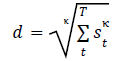
When κ=1,  submergence density is arithmetic average drawdown. When κ=∞ (or a very high number), submergence density is maximum drawdown. They use κ = 5 in examples to represent typical investor drawdown sensitivity. They define submergence risk-adjusted return as excess return (relative to the risk-free rate) minus a fraction (Θ) of submergence density, using the range 0.2 to 0.5 as reasonable for Θ. They apply submergence to several market indexes and discuss portfolio diversification and rebalancing in the context of reducing submergence overlaps. Using monthly excess returns for U.S. stocks, corporate bonds and Treasuries (S&P 500 Index, ICE BoA Corporate Bond Index and Bloomberg Treasuries Index, respectively) during 1979 through 2022, they find that:

Keep Reading

Are there different patterns of short-term stock return reversal based on stock liquidity (measured by size, volatility or turnover)? In their January 2023 paper entitled “Reversals and the Returns to Liquidity Provision”, Wei Dai, Mamdouh Medhat, Robert Novy-Marx and Savina Rizova examine interactions between short-term reversal returns and stock liquidity metrics. They select reversal candidates from the fifth (quintile) of stocks with the highest (winners) and lowest (losers) industry-relative returns over the last 1, 5 or 21 trading days, excluding 3-day returns around earnings announcements. They separately sort stocks into quintiles by size (market capitalization), volatility (standard deviation of daily returns over the last 63 days) or turnover (average percentage of shares outstanding traded daily over the last 63 days). While the sample includes all NYSE, AMEX and NASDAQ common stocks, quintile breakpoints come from NYSE stocks only. Finally, they look at returns to value-weighted intersections of reversal candidate quintiles and size, volatility or turnover quintiles. Using the specified inputs for all listed U.S. common stocks, measured monthly, during January 1973 through December 2021, they find that:

Keep Reading