Equity Premium
Governments are largely insulated from market forces. Companies are not. Investments in stocks therefore carry substantial risk in comparison with holdings of government bonds, notes or bills. The marketplace presumably rewards risk with extra return. How much of a return premium should investors in equities expect? These blog entries examine the equity risk premium as a return benchmark for equity investors.
October 21, 2016 - Equity Premium
Enterprise multiple (EM) is the ratio of enterprise value (EV) to earnings before interest, taxes, depreciation and amortization (EBITDA), with EV market value of equity plus total debt and preferred stock value minus cash and short-term investments. What happens when EM disagrees with other stock valuation metrics? In their October 2016 paper entitled “Why Do Enterprise Multiples Predict Expected Stock Returns?”, Steve Crawford, Wesley Gray and Jack Vogel investigate how EM interacts with other stock valuation metrics. They first sort stocks into fifths (quintiles) ranked by EM and then re-sort EM quintiles into sub-quintiles based on each of 12 fundamental valuation metrics: (1) financial distress; (2) O-Score (probability of bankruptcy); (3) net stock issuance; (4) composite equity issuance; (5) total accruals; (6) net operating assets; (7) momentum; (8) gross profitability; (9) asset growth; (10) return on assets; (11) investment-to-assets ratio; and, (12) a combination metric derived by first ranking stocks based on each of the 11 individual metrics and then averaging ranks for each stock. There are thus 25 double-sort portfolios for each valuation metric. They then focus on two value-weighted hedge portfolios that concentrate disagreement/agreement between EM and other valuation metrics:
- High-mispricing – long (short) stocks with low (high) EMs and high (low) fundamental valuations, representing extreme disagreement.
- Low-mispricing – long (short) stocks with low (high) EMs and low (high) fundamental valuations, representing extreme agreement.
Portfolio reformations are at mid-year annually for all variables except momentum, for which reformations are monthly. They measure portfolio performance based on monthly return, market alpha, three-factor (market, size, book-to-market) alpha and four-factor (adding momentum) alpha. Using prices and firm fundamentals required to construct specified metrics for a broad sample of U.S. common stocks during July 1972 through December 2015, they find that: Keep Reading
October 11, 2016 - Equity Premium, Volatility Effects
Does identification of trends in the CBOE Volatility Index (VIX) via simple moving averages (SMA) support effective timing of the U.S. stock market or VIX futures exchange-traded notes (ETN)? to investigate we consider timing four asset pairs:
- SPDR S&P 500 (SPY) – ProShares Short S&P500 (SH) since SH inception on 6/21/06.
- SPY – iShares 1-3 Year Treasury Bond (SHY) since 6/21/06.
- VelocityShares Daily Inverse VIX ST ETN (XIV) – iPath S&P 500 VIX ST Futures ETN (VXX) since XIV inception on 11/30/10.
- XIV – SHY since 11/30/10.
SPY and XIV are offensive assets, and SHY and VXX are defensive assets. We consider five individual SMAs to determine VIX trend: 200-day (SMA200); 100-day (SMA100); 50-day (SMA50); 20-day (SMA20); and, 10-day (SMA10). We also consider one “majority rules” combination wherein at least three of the five individual SMAs agree (SMA-Multi). When daily VIX is above (below) its SMA, expected stock market volatility is trending up (down), and we hold the defensive (offensive) asset of the above pairs. We assume a baseline 0.1% for asset switching frictions. Using daily values of the above assets as specified through most of September 2016 (10.3 years for SPY pairs and 5.8 years for XIV pairs), we find that: Keep Reading
September 30, 2016 - Equity Premium, Fundamental Valuation
Is there a straightforward way to incorporate current business/economic climate into equity market valuation ratios? In their September 2016 paper entitled “Generalized Financial Ratios to Predict the Monthly Equity Market Premium”, Andres Algaba and Kris Boudt introduce and test a generalized price-dividend ratio (GDPR) that takes into account recent business and discount rate conditions, as follows:
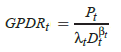
Where P is equity market (index) price, D is aggregate market dividend, the beta exponent for D accounts for changes in the kinds of companies dominating the market (those that retain versus those that pay out earnings) and the lambda multiplier for D accounts for variation in the discount rate used to evaluate dividend streams. The t subscripts indicate that all vary over time. They estimate beta and lambda via regressions using rolling historical windows of five or nine years (representing two views of business cycle length). They test the ability of GPDR to predict the U.S. equity market premium (ERP) using inception-to-date forecasting regressions, without and with a rule that switches to the historical average ERP when recent (last three and six months) GPDR predictions are poor. They use the historical average ERP as a benchmark. They employ the first nine years of data to estimate initial GPDR. They then use the next 20 years (1956-1975) for the first predictive regression, leaving 39 years for out-of-sample monthly ERP predictions (1976-2014). To assess the economic value of using GPDR to predict ERP, they consider a risk-averse, mean-variance optimizing investor who each month reallocates across equities and U.S. Treasury bills (T-bills). This investor employs a 5-year rolling window to estimate volatility, does not sell short and limits leverage to 1.5 with one-way trading friction 0.1%. Using monthly levels of the S&P 500 Index, monthly 12-month historical dividends and monthly 3-month T-bill yield as the risk-free rate during January 1947 through December 2014, they find that: Keep Reading
September 21, 2016 - Bonds, Equity Premium
How (and what) does John Bogle think about the stock and bond markets over the next decade? In their October 2015 article entitled “Occam’s Razor Redux: Establishing Reasonable Expectations for Financial Market Returns”, flagged by a subscriber, John Bogle and Michael Nolan revisit simple models for expected stock market and government bond returns first published in 1991. The stock market model distinguishes between: (1) investment return, defined as initial dividend yield plus expected annual earnings growth rate; and, (2) speculative return, defined as annual percentage change in price-to-earnings ratio (P/E). The government bond model uses the initial interest rate as a reasonable expectation for return over the life of the bond. In both models, the investment horizon is a decade. They update performances of the models to include the 25 years since publication and apply them to determine expectations for stock and bond market returns over the decade ahead. Using data for the stock market since 1871 and for 10-year U.S. Treasury notes (or equivalent) since 1915, both through 2014, they find that: Keep Reading
September 19, 2016 - Calendar Effects, Equity Premium
Does cyclic information flow from the Federal Open Market Committee (FOMC) drive equity market returns? In the June 2016 update of their paper entitled “Stock Returns Over the FOMC Cycle”, flagged by a subscriber, Anna Cieslak, Adair Morse and Annette Vissing-Jorgensen investigate interaction of the FOMC six-week meeting cycle with excess U.S. and worldwide stock market (relative to the U.S. Treasury bill). Within the FOMC meeting cycle, they look at:
- Meetings of the Federal Reserve Board of Governors and public releases of Federal Reserve book updates, statements and meeting minutes.
- Other potentially influential economic news cycles, including reserve maintenance period, macroeconomic news releases and corporate earnings announcements.
- Evidence on leaks from the Federal Reserve via media and private newsletters (with focus on Wall Street Journal articles on monetary policy).
- Public statements of Federal Reserve officials and conversations with current and former officials.
Using these data, FOMC meeting dates and daily U.S. and global (overall, developed and emerging) stock market returns, returns for individual U.S. stocks, U.S. Treasury bill (T-bill) yield and 10-year U.S. Treasury note yield during 1994 through 2015, they find that: Keep Reading
September 13, 2016 - Bonds, Currency Trading, Economic Indicators, Equity Premium
Is global diversification within asset classes disappearing as worldwide economic and financial integration increases? In their August 2016 paper entitled “Globalization and Asset Returns”, Geert Bekaert, Campbell Harvey, Andrea Kiguel and Xiaozheng Wang examine whether economic and financial integration increases global comovement of country equity, bond and currency exchange market returns. They examine three measures of return comovement for each asset class: average pairwise correlation, average beta relative to the world market and average idiosyncratic volatility. They apply these measures separately to developed markets and emerging markets. Using monthly equity, bond and currency exchange market returns in U.S. dollars for 26 developed markets and 32 emerging markets as available from various inceptions through December 2014, they find that: Keep Reading
September 7, 2016 - Equity Premium, Momentum Investing, Size Effect
Are the widely used stock characteristic/factor sorting practices of ranked fifth (quintile) or ranked tenth (decile) portfolios optimal in terms of interpretative power? In their August 2016 paper entitled “Characteristic-Sorted Portfolios: Estimation and Inference”, Matias Cattaneo, Richard Crump, Max Farrell and Ernst Schaumburg formalize the portfolio sorting process. Specifically, they describe how to choose the number of quantile portfolios best suited to source data via a trade-off between variability of outputs and effects of data abnormalities (such as outliers). They illustrate implications of the procedure for the:
- Size effect – each month sorting stocks by market capitalization and measuring the difference in value-weighted average next-month returns between small stocks and large stocks.
- Momentum effect – each month sorting stocks by cumulative return from 12 months ago to one month ago and measuring the difference in value-weighted average next-month returns between past winners and past losers.
Using monthly data for a broad sample of U.S. common stocks during January 1927 through December 2015, they find that: Keep Reading
September 1, 2016 - Bonds, Equity Premium, Strategic Allocation
A subscriber proposed adding an equity style momentum underlay to the Best Value version of the “Simple Asset Class ETF Value Strategy” (SACEVS). SACEVS each month allocates all capital to the one of the following asset class exchange-traded funds (ETF) corresponding to the most undervalued of the term, credit and equity risk premiums at prior month end, or to cash if no premium is undervalued:
3-month Treasury bills (Cash)
iShares 7-10 Year Treasury Bond (IEF)
iShares iBoxx $ Investment Grade Corporate Bond (LQD)
SPDR S&P 500 (SPY)
The proposed momentum underlay chooses SPY, iShares S&P 500 Value (IVE) or iShares S&P 500 Growth (IVW) based on highest five-month past return whenever the equity risk premium is most undervalued. Based on availability of inputs for month-end risk premium estimates, return calculations are based on closing prices for the first trading day of the next month. Using SACEVS premium estimate inputs since March 1989, first trading day of the month dividend-adjusted closes for SPY, IVE and IVW since IVE-IVW inception in May 2000 and first trading day of the month dividend-adjusted closes for IEF and LQD since their inception in July 2002, all through July 2016, we find that:
Keep Reading
May 13, 2016 - Equity Premium, Momentum Investing, Size Effect, Value Premium
How should investors think about stock factor investing? In his April 2016 paper entitled “The Siren Song of Factor Timing”, Clifford Asness summarizes his current beliefs on exploiting stock factor premiums. He defines factors as ways to select individual stocks based on such firm/stock variables as market capitalization, value (in many flavors), momentum, carry (yield) and quality. He equates factor, smart beta and style investing. He describes factor timing as attempting to predict and exploit variations in factor premiums. Based on past research on U.S. stocks mostly for the past 50 years, he concludes that: Keep Reading
May 4, 2016 - Economic Indicators, Equity Premium
Can investors exploit economic data for monthly stock market timing? In their September 2015 paper entitled “Getting the Most Out of Macroeconomic Information for Predicting Excess Stock Returns”, Cem Cakmaklı and Dick van Dijk test whether a model employing 118 economic variables improves prediction of monthly U.S. stock market (S&P 500 Index) excess returns based on conventional valuation ratios (dividend yield and price-earnings ratio) and interest rate indicators (risk-free rate, change in risk-free rate and credit spread). Excess return means above the risk-free rate. They each month apply principal component analysis to distill from the 118 economic variables (or from subsets of these variables with the most individual power to predict S&P 500 Index returns) a small group of independent predictive factors. They then regress next-month S&P 500 Index excess returns linearly on these factors and conventional valuation ratios/interest rate indicators over a rolling 10-year historical window to generate excess return predictions. They measure effectiveness of the economic inputs in two ways:
- Directional accuracy of forecasts (proportion of forecasts that accurately predict the sign of next-month excess returns).
- Explicit economic value of forecasts via mean-variance optimal stocks-cash investment strategies that each month range from 200% long to 100% short the stock index depending on monthly excess return predictions as specified and monthly volatility predictions based on daily index returns over the past month, with transaction costs of 0.0%, 0.1% or 0.3%.
Using monthly values of the 118 economic variables (lagged one month to assure availability), conventional ratios/indicators and monthly and daily S&P 500 Index levels during January 1967 through December 2014, they find that: Keep Reading